Getting started with BurnP3+
Here we provide a guided tutorial on BurnP3+, an open-source package for running spatially-explicit fire growth models to explore fire risk and susceptibility across a landscape.
BurnP3+ was designed to update and replace Burn-P3 (Parisien et al. 2005) and was developed jointly by National Resources Canada (NRCan) and ApexRMS as an open-source package within the SyncroSim software framework. Throughout the Quickstart tutorial links will be provided to the SyncroSim online documentation where applicable. For more on SyncroSim, please refer to the SyncroSim Overview and Quickstart tutorial.
This tutorial was built using the following software versions:
- SyncroSim version 3.1.29
- burnP3Plus version 2.3.0
- burnP3PlusCell2Fire version 2.2.0
BurnP3+ Quickstart Tutorial
This Quickstart tutorial will introduce you to the basics of working with BurnP3+ in SyncroSim Studio. The steps include:
- Installing the BurnP3+ package
- Creating a new BurnP3+ library
- Configuring the BurnP3+ library to:
- Running the model
- Analyzing the model results
Step 1: Installing the BurnP3+ package
Running BurnP3+ requires that the SyncroSim software be installed on your computer (version 3.1.0 or later). Download the latest version of SyncroSim here and follow the installation prompts.
In this Quickstart tutorial, you will run the BurnP3+ and BurnP3+Cell2Fire SyncroSim packages. The BurnP3+Cell2Fire package uses the Cell2Fire fire growth model.
An additional package to BurnP3+ is also available: BurnP3+FireSTARR.
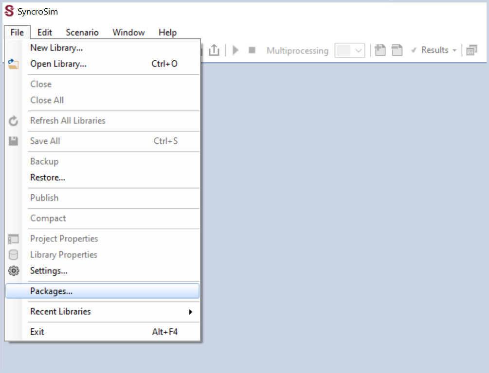
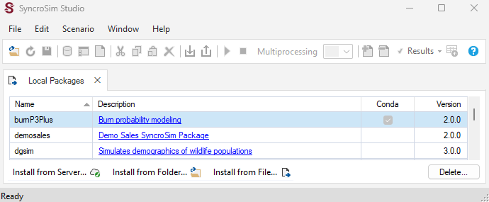
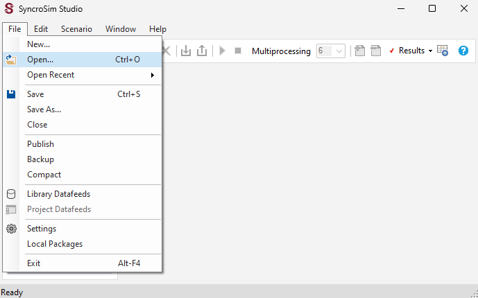
To install the BurnP3+ and BurnP3+Cell2Fire packages, open SyncroSim Studio (Start > SyncroSim Studio) and select File > Local Packages….
Click on the Install from Server… button.
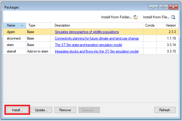
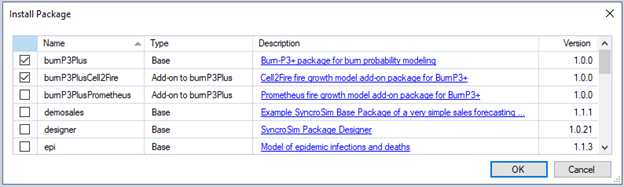
Select the checkbox beside the burnP3Plus package from the list, and click OK.
If you do not have Miniforge or Miniconda installed in your computer, a dialog box will open asking if you would like to install one of these options. Select where you would like to install conda, whether you would like to install Miniforge or Miniconda, then click Continue. Once Miniforge or Miniconda is done installing, a dialog box will open asking if you would like to create a new conda environment. Click Yes.
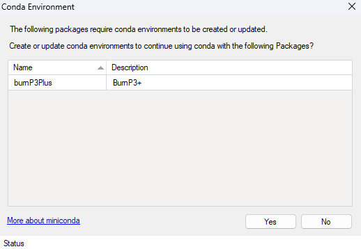
Miniforge and Miniconda are installers for conda, a package environment management system that installs any required packages and their dependencies. By default, BurnP3+ uses conda to install, create, save, and load the required environment for running BurnP3+. The BurnP3+ conda environment includes the required versions of R software and R packages that BurnP3+ was built against.
The pop-up window will close after the conda environment is created, and a checkmark will appear in the Conda checkbox beside the package description.
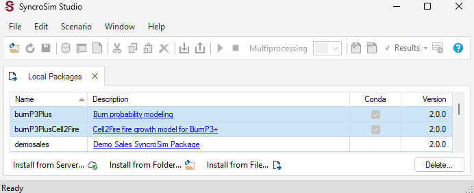
Next, click on the Install from Server… button again to open the packages repository. Select the burnP3PlusCell2Fire package from the list and click OK.
Step 2: Opening a BurnP3+ library
Having installed BurnP3+ and burnP3PlusCell2Fire, you are now ready to create your first SyncroSim library. A library is a file (with extension .ssim) that stores all the data and configurations associated with your model.
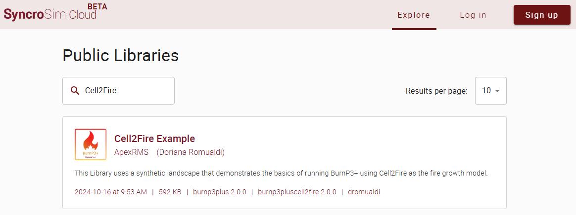
We will start with a pre-built example library using the BurnP3+ and BurnP3+Cell2Fire packages. This example uses a synthetic landscape to demonstrate the basics of running BurnP3+ using the Cell2Fire fire growth model.
To open the Cell2Fire template library in SyncroSim Studio:
-
Navigate to File > New and select From Online Template…
-
Select the burnP3PlusCell2Fire (version 2.2.0) package. Notice that the only available template is the Cell2Fire Example. Select this template library, choose a folder to save it, and click OK.
If prompted, update the library to the latest core package version. Click Apply.
-
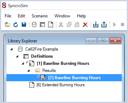
The Cell2Fire Example library will automatically open in the SyncroSim Studio Explorer window. The Cell2Fire Example library contains a project named Definitions, with one scenario named Baseline Burning Hours.
Step 3: Configuring the BurnP3+ library
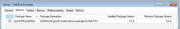
This Quickstart tutorial demonstrates the Cell2Fire fire growth model, which has already been added as a package in this template library.
This information can be found by selecting File > Library Datasheets and navigating to the General tab. Under Packages, you’ll find that the burnP3PlusCell2Fire package has been added.
Next, in the Library Explorer window, double click on Definitions. Definitions are project datasheets containing data shared across all scenarios for a project.
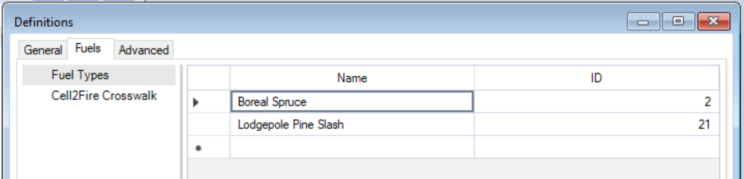
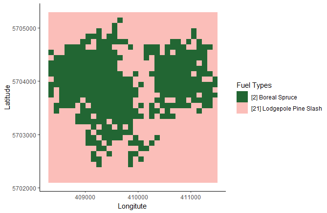
Navigate to the BurnP3+ tab, under the Fuels tab, click Fuel Types. Here, you will find a Name list for each of the fuel types present in the fuel grid, which the model requires as input. This example library already contains a fuel grid with two fuel types: Boreal Spruce and Lodgepole Pine Slash. Note that these names are free-form and can be arbitrary. Each Name is associated with an ID that must correspond to the labels given to each fuel type in the fuel grid loaded for each scenario.
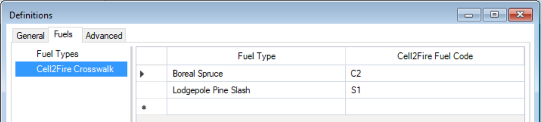
Next, under the BurnP3+Cell2Fire tab, click on Cell2Fire Crosswalk. Here, each fuel type listed under the Fuel Types tab needs to be linked to one of the fuel codes recognized by Cell2Fire. In the case of these two fuel types, Cell2Fire recognizes the Canadian Forest Service Fuel Codes C2 and S1.
Lastly, in the Library Explorer window, you will see one scenario named Baseline Burning Hours. Model inputs in SyncroSim are organized into scenarios. Each scenario is associated with scenario datasheets containing data that are specified for each scenario.
To view the model inputs for the scenario, double-click on Baseline Burning Hours.
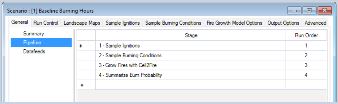
In the General tab, the Pipeline datasheet allows users to select the stages to include in the model run and their order. A full run of BurnP3+ consists of four stages:
- Stage 1: Sample Ignitions: Sample the number and locations of ignitions for each simulated burn season, or iteration;
- Stage 2: Sample Burning Conditions: Sample the burning conditions for each ignitions, which depend on when and where the ignitions occurred;
- Stage 3: Grow Fires with Cell2Fire: Simulate each fire deterministically using a fire growth model; and
- Stage 4: Summarize Burn Probability: Summarise the outputs of the fire growth model to calculate burn probability and other burn metrics.
In this example, we will run the full pipeline.
In the BurnP3+ tab, Run Control allows users to specify the number of iterations or Monte Carlo realizations to run. In this example, each scenario will run for 100 iterations. Each iteration represents a stochastic simulation of a single fire season. Typically, BurnP3+ should be run for tens of thousands of iterations.
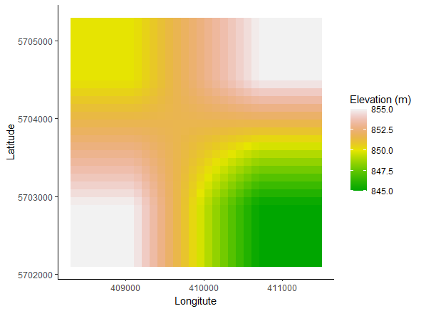
The Landscape Maps contains the pre-loaded raster files for Fuel and Elevation (although this is an optional input).
Raster files for Fire Zone and Weather Zone are optional and will not be considered in this Quickstart tutorial. These raster files allow end users to stratify the landscape and define different statistical distributions for model inputs and summarize model outputs according to these zones. For example, daily weather may vary according to Weather Zone.

The following four tabs contain the rules for stages 1 to 4.
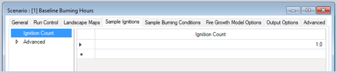
Stage 1: Sample Ignitions
Expand the Sample Ignitions node. The Ignition Count datasheet defines the number of fires that should be ignited every iteration within a season. For the purposes of this Quickstart tutorial, Ignition Count was set to 1.
Stage 2: Sample Burning Conditions
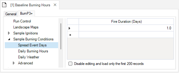
Navigate to the next node, Sample Burning Conditions. The Spread Event Days datasheet specifies the number of days uncontrolled fires are actively burning and spreading in a season. Similarly, for the purposes of this Quickstart tutorial, Spread Event Days was set to 1 for all Seasons.
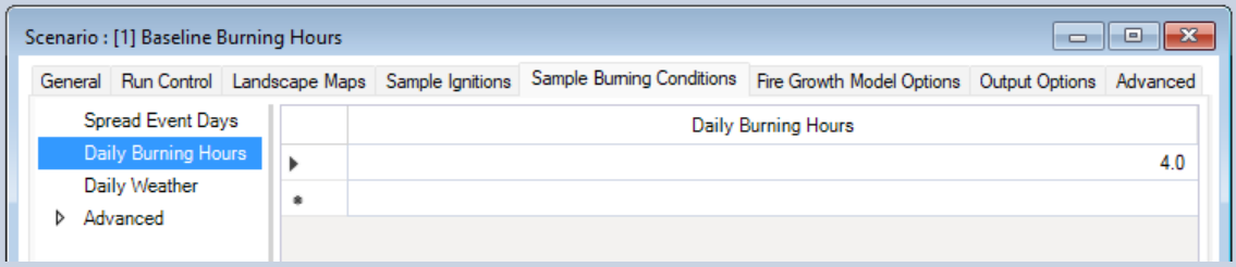
The Daily Burning Hours datasheet defines the number of hours fires are actively burning per day. For the Baseline Burning Hours scenario, Daily Burning Hours was set to 4 for all Seasons.
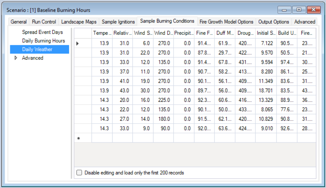
The Daily Weather datasheet specifies weather variables for the landscape of interest. Each row corresponds to one day of weather data for a given season. The required variables are: temperature, relative humidity, wind speed, wind direction, precipitation, fine fuel moisture code, duff moisture code, drought code, initial spread index, buildup index, and fire weather index.
Stage 3: Grow Fires with Cell2Fire
Under the Fire Growth Model Options tab, all settings are optional. As advanced features, they will not be covered in this Quickstart tutorial. By leaving the Fire Growth Model Options empty, BurnP3+ will use the default values.
Stage 4: Summarize Burn Probability
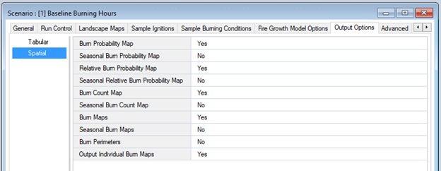
Finally, the Output Options node specifies which outputs will be generated after running the scenario. The option to output the Fire Statistics Table in the Tabular Output Options datasheet is set to Yes (default). The options to output the various seasonal maps in the Spatial Output Options datasheet are set to No since there is no seasonal stratification in this model. Additionally, the Burn Perimeters are also set to No because this option is not provided by Cell2Fire.
Note: If all rows in the Spatial Output Options datasheet are left blank, BurnP3+ will default to generating all spatial outputs. However, if only some rows are set to return spatial outputs, the model will only return outputs for the specified rows.
Close the window for the Baseline Burning Hours scenario.
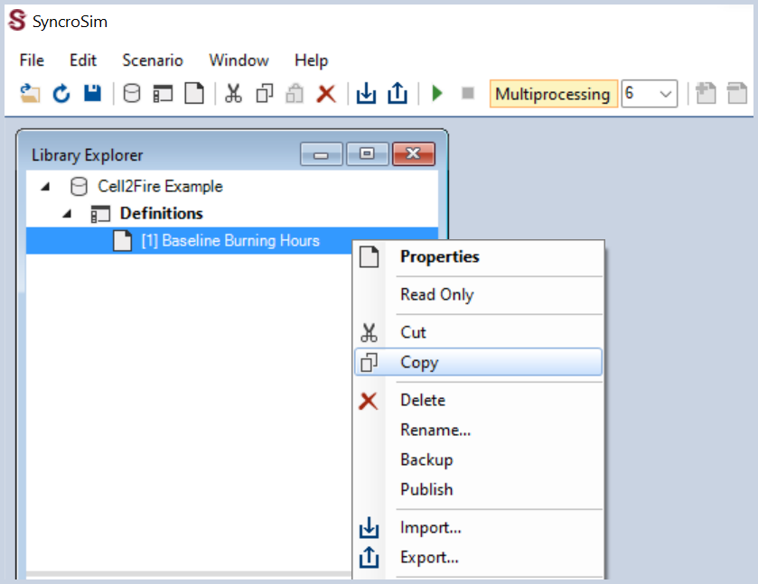
Next, you will create a new scenario to compare the effects of Daily Burning Hours on burn probability. While you could create a new empty scenario, instead you will copy, paste, and modify the existing scenario to save time and reuse the model inputs. To copy an existing scenario, right-click on the Baseline Burning Hours scenario in the Explorer window, and select Copy from the context menu.
Next, right-click in the Explorer window and select Paste from the context menu.
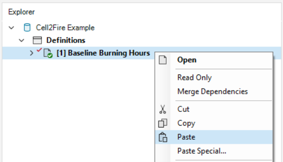
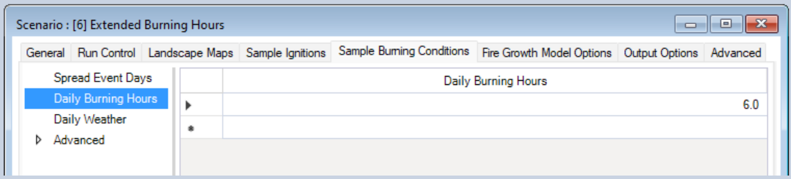
Rename the scenario by right clicking the newly created scenario, selecting Rename… from the context menu, and typing Extended Burning Hours. Next, double click on the Extended Burning Hours scenario and navigate to the Sample Burning Conditions tab. Here, you will modify the input Daily Burning Hours from 4 to 6.
Step 4: Running the Model
After reviewing the model inputs and creating a new scenario, you are now ready to run the model.
Multiprocessing is enabled to run 6 jobs in parallel. You can adjust the number of multiprocessing jobs according to the specifications of your computer. A good rule of thumb to follow is number of logical cores minus 1.
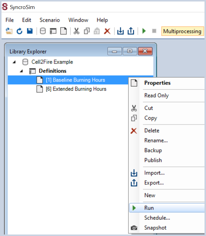
Next, right-click on the Baseline Burning Hours scenario, and from the context menu select Run. If prompted to save your project, click Yes.
A Run Monitor window will appear, indicating the Status of the scenario as Running. At the bottom of the SyncroSim Studio window, an orange progress bar will provide further information during each stage of the pipeline.
When the run has completed the Status will change to Done in the Run Monitor window. If an error or warning has been issued, click on the Run Log link to see a report of problems. Make any required changes to your scenario and re-run it.
Running a model in SyncroSim produces a results scenario, which contain the input datasheets associated with the parent scenario, as well as output datasheets for the scenario run. Each results scenario inherits the parent scenario’s name and receives a unique ID.
Repeat the same process to run the Extended Burning Hours scenario.
Step 5: Analyzing the Model Results
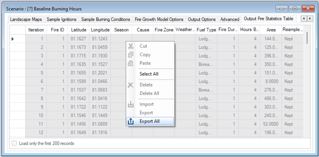
To view the tabular results from each of your runs, double-click on one of your results scenarios and navigate to the last datasheet in the BurnP3+ tab, called Output Fire Statistics Table. Here, you can view the information about every fire that was run during the simulation. You can also easily export the data to a CSV or Excel file by right-clicking anywhere on the spreadsheet, and selecting Export All from the context menu.
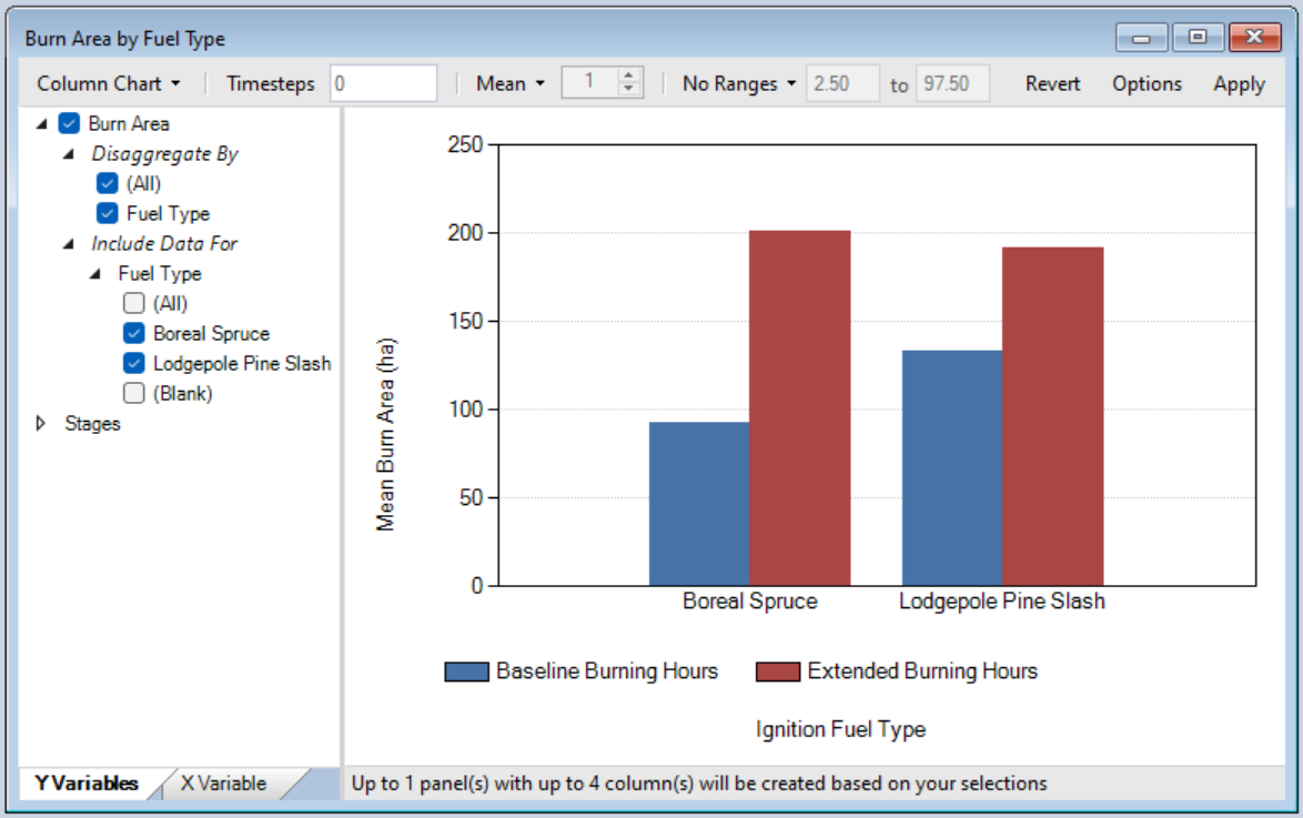
Next, move to the results panel at the bottom left of SyncroSim Studio. Under the Charts tab, double-click on Burn Area by Fuel Type to see the tabular results for area burned.
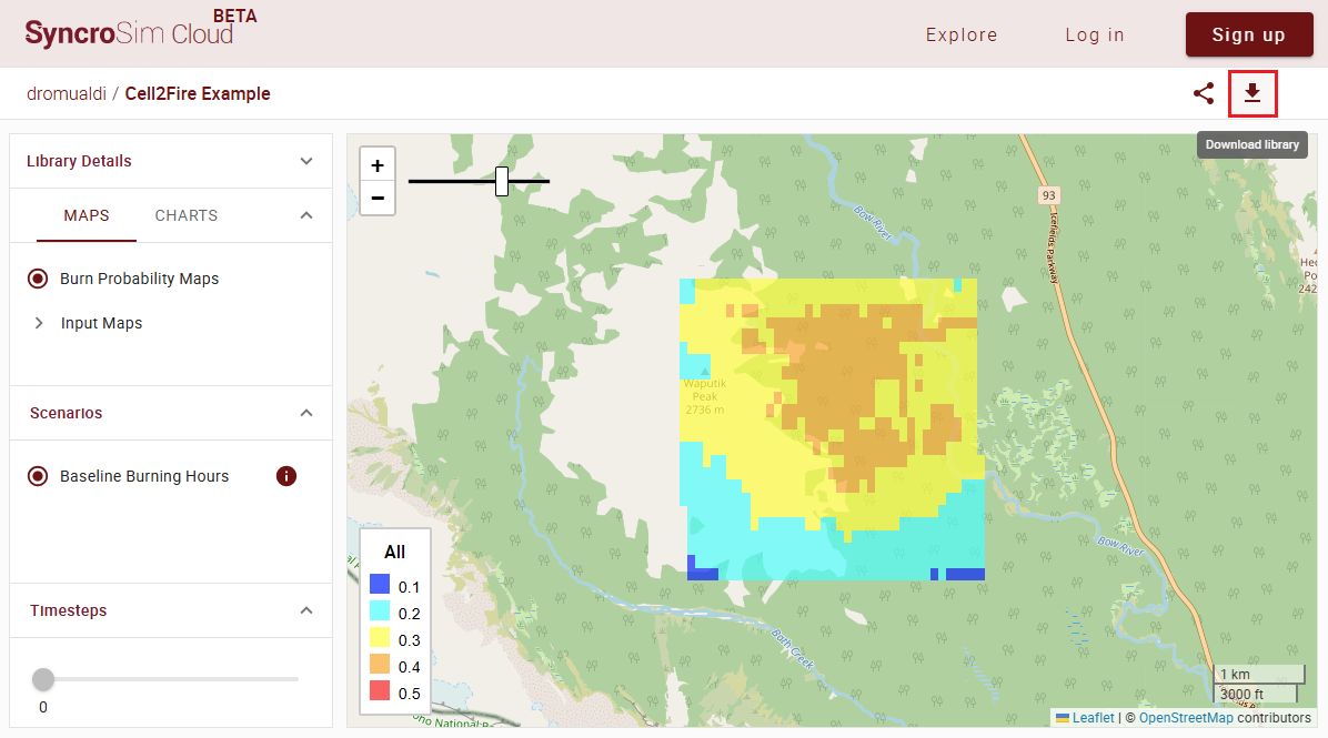
Next, navigate to the Maps tab and double-click on Burn Probability Maps.
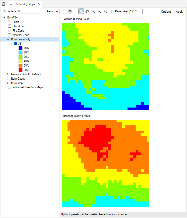
Note: Map legends can be customized by double-clicking on the legend entries. You can also add or remove a results scenario from the charts and maps by right-clicking on the results scenario in the Library Explorer, then choosing either Add to Results or Remove from Results from the context menu. Scenarios with results currently selected for analysis have a red checkmark and are bolded in the Library Explorer.